Dissolving shapefiles using shapely and psycopg2

Geospatial data is commonly stored in PostgreSQL which, through PostGIS, provides a great set of tools for geospatial analysis. However, if this analysis is part of a larger workflow chain it can sometimes be easier to work with the excellent shapley package that provides a easy set of calls for advanced geospatial analysis. The script below looks at how to extract data from PostgreSQL, insert into shapely and run a common geospatial query: dissolve (cascaded union).

#!/usr/bin/python
import psycopg2
import shapely.wkb as wkb
import shapely.wkt as wkt 
from shapely.ops import cascaded_union
import json
 
def main():
    
    #Define our connection string
    conn_string = "host='12.34.56.78' dbname='nathan_local' user='postgres' password='XXXXXXXXX'"
 
    # print the connection string
    print("Connecting to database %s" % (conn_string))
 
    # get a connection
    conn = psycopg2.connect(conn_string)
 
    # conn.cursor will return a cursor object, you can use this cursor to perform queries.
    cursor = conn.cursor()
    print("Connected!\n")

    # use the cursor object to extract data from postgreSQL
    cursor.execute("SELECT tile_name, st_asewkt(wkb_geometry) FROM test.tablename")

    tiles = list(cursor.fetchall()) #fetchall returns all matching records

    coverage = {}
    for name, geometry in tiles:
        coverage[name] = wkt.loads(geometry.split(';')[1])

    geometry = cascaded_union(coverage.values())
	
    with open('/file/path/test.json', 'w') as outfile:
        json.dump(mapping(geometry), outfile)
	 
if __name__ == "__main__":
	main()

Processing OS Mastermap topography dataset

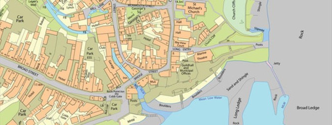
OS MasterMap Topography Layer is the most detailed and accurate view of Great Britain’s landscape – from roads to fields, to buildings and trees, fences, paths and more. It contains over 470,000,000 topographic identifiers (TOIDs) providing the user with a unparalleled view of Great Britain. With this sheer volume of detail comes ALOT of data and this post will explore two tools for uploading the whole dataset into PostgreSQL.

The product normally comes on a set of CD-ROMs (11 for the whole dataset) and it is essential that you get hold of the Feature validation Dataset (FVDS) which provides a list of all the TOID’s so you can cross reference with what has been uploaded.

I have also created a layer that contains 1x1km grid squares that have OS MasterMap topography data (244,583 in total) by using a combination of this free tool and the OS 1km price matrix. This is useful as a reference to check you have the data everywhere you should do and also if you need to use the grid squares as a search mechanism for the data.

You can download this layer from here.

OS Translator II

Developed by Lutra consulting and available as a QGIS plugin, this tool provides a simple GUI for uploading data. It allows data to be uploaded with styles and provides postgres setup details to optimise the speed of upload. The downside is that the tool only supports create or replace (not APPEND) which implies COUs might not load consistently.

To use you need to be connected to your postgres database through the QGIS DB manager. You are presented with a variety of options: you will definitely want to create a spatial index and remove duplicates because we are dealing with geographic chunks of data. The last two options relate to styling the layer and it is recommended to select these aswell. Two additional fields will be added allowing you to style the layer with either ESRI, Geoserver or QGIS stylesheets. In the right window you can also select the fields you want to be entered – the less you select the quicker the upload but at the cost of losing data.

I had one issue with the styling and had to add these fields after the initial upload. I believe this was to do with the svg path not being correct (as mentioned here. If you experience the same issues then just download the SQL scripts for schema 7 here and schema 9 here. Note, you will need the array SQl scripts as items under the styling columns are stored in array’s.

You can see the visual difference between schema 7 (bottom) and schema 9 (top) below:

Astun loader

The Astun loader has one significant advantage (it can append records meaning COUs can be handled) and one significant disadvantage (it’s alot slower) than the OS translator. Therefore, you could use the OS translator to get the whole dataset in PostgreSQL and then use Astun to handle the COU’s for example.

This tool allows GML/KML data in general (OS Mastermap is GML) to be transferred to any format compatible with OGR – in this case we will transfer the data into PostgreSQL. To be this we need to create a config file, some examples are provided here. The one I used is presented below:

# Note: Environment variables can be used with any of
# the options by using a token of the form:
# $HOME, ${HOME} or %TEMP% (Windows only)

# The directory containing your source files.
# All supported files in the specified directory and
# it's descendants will be loaded.
src_dir=/home/brainnwave_nathan/Desktop/hp/2255669-HP4500-5c11.gz

# The directory used to store the translated data
# if writing to a file based format such as ESRI
# Shape, MapInfo TAB etc.
out_dir=/home/brainnwave_nathan/Desktop/Output

# The directory used to store temporary working files
# during loading.
tmp_dir=/home/brainnwave_nathan/Desktop/temp

# The ogr2ogr command that will be used to load the data.
# Here you can specify the destination format and any
# associated settings (for example database connection
# details if you are writing to PostGIS).
# As well as environment variables the following tokens can
# be used which will be substituted at runtime:
# $output_dir - the directory specified by the out_dir setting
# $base_file_name - the file name of the file to be loaded
# $file_path - the full path of the file to be loaded
ogr_cmd=ogr2ogr --config GML_EXPOSE_FID NO -append -skipfailures -f PostgreSQL PG:'dbname=brainnwave active_schema=public host=12.34.56.78 user=postgres password=abcdefghij' $file_path

# The command used to prepare the source
# data so it is suitable for loading with OGR. Choose a prep
# class appropriate for your data, for Ordnance Survey
# products take a look at prep_osgml.py for the available classes.
prep_cmd=python prepgml4ogr.py $file_path prep_osgml.prep_osmm_topo

# An optional command to be run once OGR has created it's output.
# Called once per file, useful for loading SQL dump files etc.
# All of the tokens available to the ogr_cmd can be used here.
post_cmd=

# Optional OGR .gfs file used to define the
# feature attributes and geometry type of
# the features read from the GML.
gfs_file=../gfs/osmm_topo_postgres.gfs

# Whether to output debug messages and keep
# temporary files (True or False).
debug=True

Once the data is loaded, the SQL scripts to append style fields still have to be run to allow the use of stylesheets.

GDAL / OGR cheatsheet

A wonderful cheatsheet for using GDAL and OGR – taken from Derek Watkins GitHub page

Vector operations

Get vector information

ogrinfo -so input.shp layer-name

Or, for all layers

ogrinfo -al -so input.shp

Print vector extent

ogrinfo input.shp layer-name | grep Extent

Inserting EA WMS layers into OpenLayers

The Environment Agency have provided lots of very useful data under the OGC WMS. To get this into OpenLayers, you need two pieces of information.

Firstly, there is a URL provided at the bottom of the page:

http://www.geostore.com/OGC/OGCInterface?SERVICE=WMS&INTERFACE=ENVIRONMENT&LC=0

In addition to this, we need the layer name that you would like to view. To find these we need to add the following to the URL:

&VERSION=1.1.1&REQUEST=GetCapabilities

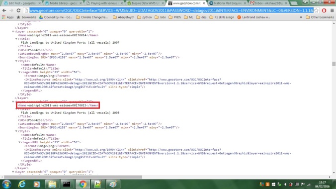
This will then open the following XML:

The red box highlights the branch you are searching for.

Once you have the name, you can use the code below to add the layer.

var ea_wms = new ol.layer.Tile({
              source: new ol.source.TileWMS({
                  url: 'http://www.geostore.com/OGC/OGCInterface',
                  params: {"SERVICE": "WMS",
                           "UID": 'UDATAGOV2011',
                           "PASSWORD": "datagov2011",
                           "INTERFACE": "ENVIRONMENT",
                           "LC": "0",
                           "LAYERS": "eainspire2011-wms-eaieaew00170015"
                           }
               })
});

The UID, PASSWORD, INTERFACE and LC all come from the initial URL with the LAYERS parameter indicating the name of the layer you wish to import. You can then see the layer on your map.

Open Layers web map development with Geoserver

The last few months, I have been learning the basics of OpenLayers 3.6. This has involved learning to setup a map, import layers from various sources and add feature overlays.

The screenshots below show where I am at: I have a few layers (one geojson, WMS on my own geoserver and a WMS on a public geoserver) which can be switched on and off and a feature overlay for the Countries layer, providing the user with some relevant information. Screenshots can be seen below.

All layers on, with feature overlay on France and text occuring in bottom right hand of screen.

Counties layer (my geoserver) switched off, with additional feature overlay styling upon specified zoom layer.

Streams layer (public geoserver) and OSM base map switched on, other layers off.

Source code can be seen below:

Calculating number of overlaps between polygons

A common application within GIS is to create buffer / catchment areas – an interesting analysis is then to see how many overlaps occur with the each catchment indicating whether a site is under or over provisioned. This can be achieved using Postgis and the following fantastic tutorial.

This can you allow you to produce maps like the following:

Below gives a snapshot of the process:

create table boundaries_allot as select ST_Union(ST_ExteriorRing(geom)) from
(select (ST_DumpRings((st_dump(geom)).geom)).geom as geom from allotment_buffer) q 

This has been altered from the tutorial to include multi polygons. ST_Dump breaks down multi polygons into single polygons and ST_DumpRings provides the interior and exterior rings of polygons (for complex polygons)

CREATE SEQUENCE polyseq_allots;
CREATE TABLE polys_allots AS
SELECT nextval('polyseq_allots') AS id, (ST_Dump(ST_Polygonize(st_union))).geom AS geom
FROM boundaries_allot;

This creates individual polygons for each multi-linestring and uses ST_Dump to switch any multi polygons to single polygons.

ALTER TABLE polys_allots ADD COLUMN count INTEGER DEFAULT 0;
UPDATE POLYS_allots set count = p.count
FROM (
  SELECT count(*) AS count, p.id AS id  
  FROM polys_allots p 
  JOIN allotment_buffer c 
  ON ST_Contains(c.geom, ST_PointOnSurface(p.geom)) 
  GROUP BY p.id
) AS p
WHERE p.id = polys_allots.id;

Once we have the individual polygons, by using the centroids of the new small polygons with the set of original circles, we can calculate how many circles contain each centroid point.

Creating ArcMap tools using python scripts: ASCII to Raster batch processing

Recently, I had to process 400 tiles of LiDAR data and find a method that would allow beginners to GIS to achieve the same in the future. For this I decided to create a custom tool in ArcMap which uses a python script to batch process the ASCII files in rasters and then merges these into a final DEM. The users can then start processing this layer for their individual needs.

Script:

# Import system modules
import arcpy, os, sys

# Set local variables

inASCII = str(sys.argv[1]) #these variables are linked to the data the user will input when running the tool.
outRaster = str(sys.argv[2])
mergeGeodatabase = str(sys.argv[3])
outputFilename = str(sys.argv[4])
rasterType = "FLOAT"
emptyString = []
britishNationalGridprj = "PROJCS['OSGB 1936 / British National Grid',GEOGCS['OSGB 1936',DATUM['D_OSGB_1936',SPHEROID['Airy_1830',6377563.396,299.3249646]],PRIMEM['Greenwich',0],UNIT['Degree',0.017453292519943295]],PROJECTION['Transverse_Mercator'],PARAMETER['latitude_of_origin',49],PARAMETER['central_meridian',-2],PARAMETER['scale_factor',0.9996012717],PARAMETER['false_easting',400000],PARAMETER['false_northing',-100000],UNIT['Meter',1]]"

#Set path names and convert from windows to python

inASCII_convert = inASCII.replace('\\','//')
outRaster_convert = outRaster.replace('\\','//')
mergeGeodatabase_convert = mergeGeodatabase.replace('\\','//')

#Convert from ascii to raster for each individual file

for files in os.listdir(inASCII_convert):
	if files.endswith(".asc"):
		arcpy.ASCIIToRaster_conversion(inASCII + "//" + files, outRaster + "//" + files.replace(".asc",".tif"), rasterType)
	
#create string for raster mosaic

for outputs in os.listdir(outRaster_convert):
	if outputs.endswith(".tif"):
		emptyString.append(outRaster_convert + "//" + outputs)
	outputString = ';'.join(emptyString)
	
#merge all tiffs together
	
arcpy.MosaicToNewRaster_management(outputString, mergeGeodatabase_convert, outputFilename, britishNationalGridprj ,"16_BIT_UNSIGNED","" , "1","" ,"" )

Creating a tool in ArcMap:

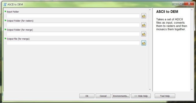
Using ArcCatalog, find the location where you want the toolbox and right-click to select ‘New Toolbox’. From here go to Add -> Script and follow the prompts. When you reach the properties page we need to select four pieces of information the user enters to relate to the 4 inputs that were specified in the script using the sys.argv command. Note these need to be in the same order. Choose a name for the input, select whether it is a input/output in the environment property and then select the type.

The first two relate to folders where all the files are stored, the third to the folder where the output is stored and the forth is for the output file name.

Now you can can run the tool just like any others in toolbox.

QGIS Time manager

Time manager is a fantastic plugin allowing you to create a time lapse video of geospatial data provided it comes with a date-time attribute. The following video shows data on where energy advice visits took place using the created date time stamp from the survey plotted every 24 hours.

PG routing – driving distance

Building on the work of previous posts looking at building routable networks and finding the shortest path in a network, this post will look at creating buffers around nodes based on a cost attribute specifed by the user.

The driving distance function, which comes with pg routing 2.0, creates an alpha shape around a node, normally based on the distance someone could travel from that node, or how far someone could go in a time interval.

For this example, we are looking at where someone could travel in 1km along the network from a central node. The following query selects all the nodes that are within 1 km of node 2000.

PG routing – shortest path algorithms

Once a routable network has been set up we can start to find the shortest path (using Dijkstra’s algorithm) between two points. From here on, I will be using the OSM data for the London road network.

The query use’s a ‘cost’ column – which could be anything thing you like – to calculate the shortest cost from one node to another. In this example I decided to use travel time (rather than distance).

First, I changed the distance of each vertex (the way table) from km to miles, and then calculated the time it would take to traverse each vertex whether walking, cycling or driving. To make this more accurate, I updated the max speed (forward and backward) along each vertex dependent on its class (as listed in the class table).